Aligning Short Reads to Reference Sequences
After trimming and filtering .fastq files for quality, the next step in preparing data for analysis is aligning those reads to a reference—a previously-assembled set of DNA sequences of known identity that include the genomic regions in your short-read data. Depending on your goals and library preparation, a reference sequence may be an entire genome, or a single gene. It may be from an individual of the same species as the samples in your dataset, or a related species you didn’t sequence (though there are impacts to choosing too-divergent a reference; see Rick et al. 2024). For our example data, we will use the sequences used to generate oligonucleotide probes for target capture of the seven hemoglobin subunits. (These probes were generated from an annotation of the Sicalis [luteiventris] luteola genome—another member of Thraupidae.
Indexing a Reference Sequence
Regardless of sequencing platform, assembled DNA sequences are typically stored in the .fasta format. These plain text files have a simple structure and are easier to interpret than the .fastq files you inspected the previous week. Let’s take a look at the reference .fasta we’ll be using:
head -n 4 bioe-591-genomics/course-materials/data/references/hemoglobin_references.fastaThis command should produce the following output (though note that you can extend or shorten this preview by varying the -n argument):
>HBAA_Sicalis_luteiventris
NGGCTCCAGCAGCCCCGAGCCGGGCGGAGCCCCAGCACCGCATATAAGGGCGGCGGCGGGCAGCGGGGACACCCGTGCTGGCGCTGCCGACTCGGAGGTGACACCATGGTGCTGTCCGCCGCCGACAAGACCAACGTCAAGGGCGTTTTCGCCAAAATCGGCGGCCAGGCCGACGAATATGGCGCCGATGCCCTGGAGAGGTATCGTGGCTGTCCCCTGTGTGACCCTCTCTCTCCTCTCCAGCCCCGACTCCCTCGCATCTGCCCCCTCTTGTCCCCATCCGCTGCTGTCCTTTGCCACCCTGTCCCTGTCTCACCTGTCTCTGAACCCCTTTGTTCTGCAGGATGTTCGCCACCTACCCCGCCACCAAGACCTACTTCCCCCACTTCGACCTAGGAAAGGGCTCTGCCCAGGTCAAGGGGCACGGCAAGAAGGTGGCAGGAGCACTGGTGGAAGCTGTCAACCACATCGATGACCTTGCTGGTGCCCTCTCCAAGCTCAGCGACCTCCACGCCCAAAAACTCCGTGTGGACCCTGTCAACTTCAAAGTGAGTGTCTGGGGAGGGGTGACCAGCCCAGCTTCCCTCCTGCACCTCTTGGCTACTGCCTCGCCTCATTCCCTTGCTCACCACATCGTTTTGCCTTCCAGCTGCTGGGCCAGTGCTTCCTGGTGGCGGTGGCCACCCGCAACCCCGGTCTCCTGACCCCAGAGGTCCATGCTTCCCTGGACAAGTTCCTGTGTGCCGTGGGCACCGTGCTGACTGCCAAGTACCGTTAAGGCGTGTGCTGTGGCCAGAGCTGGAGCCGACACCCCACCAGCCCTCCGACAGCCAGCAGTCAAATGTCCTGAAATAAAATCTCTTGCATTTGTGCTGCAGCT
>HBAD_Sicalis_luteiventris
ATGCTGACCGCCGAGGACAAGAAGCTGATCCAGCAGATGTGGGGAAAGCTGGGCGGCGCCGAGGAGGAAATCGGAGCCGAGGCCCTGACGAGGTACAGACCCGGGGACCCCATGGGAGAGGGGACAAGGGGGTGGGAGCCCCACGGAGGGGCCGGCATGGTGGGTCCAGCTGGGGTCAGCACCACTGACTGTCCCACTCTCCCAGGATGTTCTGCTCCTACCCCCCGACCAAGACCTACTTCCCCCACTTCGACCTGTCCCCGGGCTCTGACCAGGTCCGTGGCCATGGCAAGAAAGTGGTGGCTGCCCTGAGCACTGCCATCAAGAACATGGACAACCTCAGCCAGGCTCTGTCTGAGCTCAGCAACCTGCACGCCTACAACCTGCGTGTGGACCCCGTCAACTTCAAGGCAGGCAGGGGGAATGGGGGTGGGGAATGGGGACAGGGAGCAGAATGGGGGGACAGGGAGCAGGGGACGGGGAATGGATACTGAGGGACAGGGAATGGGGCACAGGGATCGGGATGGGAGCCGGGGGATGGAGGACGGGAGATGGGGGAGGGTGGACGGCAGGGGATGGGGTACAGGGGCTGTGGGACAGGGACCGGGATGGGGACATCGGTGCTAAGGCCCCTTTTTCCTTGCAGTTCCTGTCGCAGTGCTTGCAGGTGGCGCTGGCTACCCGCCTGGGTAAGGACTACAGCCCCGAGGTGCACTCTGCCGTCGACAAGTTCATGTCGGCCGTGGCCAGCGTGCTGGCTGAGAAGTACAGATGA
In .fasta files, each contiguous sequence—here exons or genes, but often analogous to chromosome-scale chunks of thew genome—is prefaced by a carrot (>) and an identifier. We can see the name of two hemoglobin-A subunits (\(\alpha\) and \(\delta\)), followed by the name of species they were extracted from. The subsequent text (which is all on a single line, despite how it appears in this window) is simply the sequence itself. Most bases are our familiar abbreviations for adenine, cytosine, guanine, and thymine, but note the presence of “N”, which indicates the base in its position may be any of the previous nucelotides. (This is an example of an ambiguity code, something you should passingly familiarize yourself with here).
When we align our short read .fastq data to this reference—more properly, these reference sequences—some will map to the contiguous sequence in >HBAA_Sicalis_luteiventris, some will map to >HBAD_Sicalis_luteiventris, and others will map to the exons farther down in the file. To prepare for this step, we need to index these files. Confusingly, we need to do it twice, with two different tools (bwa and samtools) for two different purposes: 1) generating the alignment itself, and 2) reading / editing / viewing it. We will start by creating a .yaml for a Mamba environment named align that contains the software we need:
name: align
channels:
  - conda-forge
  - bioconda
dependencies:
  - bwa=0.7.17
  - samtools=1.19
mamba env create -f align.yamlIndexing for alignment uses a software package called bwa, an abbreviation for “Burrows-Wheeler Aligner”, itself named for the underlying algorithm it employs. Though the project’s home on the internet has become concerningly dated-looking, bwa remains a standard, ubiquitous tool in bioinformatics. Take a minute and scan bwa’s documentation. The structure of the commands and arguments should look familiar; as we will be using bwa index and bwa mem, it is worth spending more time on those sections of the manual. Indexing for reading and visualizing our alignment uses samtools; its documentation is here.
Recall that you are on the log-in node, and that you are unable to write in the course-materials/ subdirectory, so you will have to adjust the paths of output files accordingly (and / or copy the reference sequence to your own directory if needed). Once again, we will need to create an .sbatch script in order to run our indexing commands. At this point, I expect you to be able to adapt your previous templates to account for new paths, new Mamba environments, and new job names / .out and .err file names. Because we have installed bwa and samtools in the same environment, you may run them sequentially in the same SLURM job, or run two separate jobs—whatever works best for your brain and workflow.
As detailed in the documentation, indexing for alignment with bwa uses the command bwa index and a path to the relevant reference sequence(s):
bwa index reference.fastaIndexing with samtools is nearly identical:
samtools faidx reference.fastaOnce you have adapted these commands to your data and called your .sbatch script, they will produce a suite of output files with the same suffix as our reference (hemoglobin_references.*). For now, we will look only at the output of samtools indexing: hemoglobin_references.fai. Because we only have seven exons in our file—where a full reference genome might have thousands of contigs or scaffolds, ranging from chromsome-sized sequences to tiny misplaced fragments—we can do this with cat instead of head:
cat hemoglobin_references.fasta.fai HBAA_Sicalis_luteiventris 880 27 880 881
HBAD_Sicalis_luteiventris 775 935 775 776
HBB2_Sicalis_luteiventris 2272 1738 2272 2273
HBB_Sicalis_luteiventris 1358 4037 1358 1359
HBE_Sicalis_luteiventris 1559 5422 1559 1560
HBPI_Sicalis_luteiventris 1910 7009 1910 1911
HBRH_Sicalis_luteiventris 1143 8947 1143 1144Here, the columns refer (in order) to 1) the contig name (here, our exons); 2) the number of bases in the contig (note the range!); 3) the byte index of the file where said contig begins (think “coordinate the computer uses to find the start of the sequence, where spaces, nucleotides, and newline indicators all get a position”); 4) the number of bases per line in the .fasta; and 5) the number of bytes per line (usually one more than the number of bases, as there is an invisible new line character / byte).
Aligning Reads
Once your reference sequences are index, you are ready to align your reads with bwa mem, a command that takes as its bare-minimum arguments a pair of reads corresponding to a particular sample and outputs a .sam file, a suffix that stands for Sequence Alignment/Map (SAM) format. This job will be the most computationally intensive we have run to date, and as a result, you will likely want to boost the run time beyond 10 minutes. (While preparing this lesson, my command for a single individual took about 5 minutes to complete.)
Create a new .sbatch script that will load your align Mamba environment and then call the following command (with paths and sample names edited to reflect directory permissions and your own species and IDs):
bwa mem -t 4 hemoglobin_references.fasta species_ID_R1_001_trimmed.fastq.gz species_ID_R2_001_trimmed.fastq.gz > species_ID.samNote that I have added an optional argument (-t 4), which sets the number of threads (=independent processes) that bwa will call to four. For larger jobs, this can substantially speed up runtime, as bwa can parallelize its operations, i.e. align reads to different regions of the reference sequence simultaneously. In the current case, it is unlikely to have a major impact, but tweaking this appropriately is key for large datasets. Instructions relevant to this command can be found in the manual, or by typing bwa mem with your align environment active:
-t INT number of threads [1](Here, INT refers to the argument input type need (an integer); the number in brackets is the default, a convention used widely.)
Once your command is running, use sacct or squeue -u $USER to check the status of the job. You can also see bwa’s voluminous output in semi-real time by typing tail or cat followed by the name of your .err file.
Viewing and Reading Alignments
Once bwa has finished running, examining the output will help shed light on the alignment (=read mapping) process. Sequence Alignment/Map files are tab-delimited plain text, with an optional header section (each line with an @ character) and then an alignment section, where each line contains a read prefaced by data stored a set of standardized fields. The details of these fields are technical and mostly beyond us—check out this Wikipedia article if you are curious—but include key information on which sequence a read mapped to, where on the sequence it mapped, and how well it fit there. Because .sam files are plain text, we can look at them with head or cat (e.g., head sample.sam):
@SQ SN:HBAA_Sicalis_luteiventris    LN:880
@SQ SN:HBAD_Sicalis_luteiventris    LN:775
@SQ SN:HBB2_Sicalis_luteiventris    LN:2272
@SQ SN:HBB_Sicalis_luteiventris LN:1358
@SQ SN:HBE_Sicalis_luteiventris LN:1559
@SQ SN:HBPI_Sicalis_luteiventris    LN:1910
@SQ SN:HBRH_Sicalis_luteiventris    LN:1143
@PG ID:bwa  PN:bwa  VN:0.7.17-r1188 CL:bwa mem -t 4 hemoglobin_references.fasta /home/k14m234/bioe-591-genomics/course-materials/data/raw_reads/Oreomanes_fraseri/Oreomanes_fraseri_159769_R1_001.fastq.gz /home/k14m234/bioe-591-genomics/course-materials/data/raw_reads/Oreomanes_fraseri/Oreomanes_fraseri_159769_R2_001.fastq.gz
J00138:88:HG7TGBBXX:3:1101:5365:1086    77  *   0   0   *   *   0   0   NTTAAAAAAAAAGGATGCATCTAAGGACAATGACAGGGATGAAATGTTTCTTTCTATAATGTCTGAAAAGCCATGGTCTTTGGGGAAGGTTCTTAAATTCTGAAAATAGGGAAAGTCACACCAATTCAGGTTCAAGATCCAGGATAGCCTA#AAFFJJJJJJJJJJJJJJJJJJJJJJJJJJJJJJJJJJJJJJJJJJJJFJJJJJJJJJJJJJJJJJJJFJJJJJFJJJJJJJJJJJJJJJJJJJJJJJJJJJJJJJJFJJJJJJJJJJJJJJJJJJJJJJJJJJJJJJJJJJJJJJJJJJ  AS:i:0  XS:i:0
J00138:88:HG7TGBBXX:3:1101:5365:1086    141 *   0   0   *   *   0   0   NTATAATTAGGAGAGCATAGACACAAGTATTTTCACCAAAGGAATTCCAGGTTCTCCAGTCAAAATTAATATTCGTTCCTAGATAGGCTATCCTGGATCTTGAACCTGAATTGGTGTGACTTTCCCTATTTTCAGAATTTAAGAACCTTCC#AAFFJJJJJJJJJJJJJJJJJJJJJJJJJJJJJJJJJJJJJJJJJJJJJJJJJJJJJJJJJJJF<JJJJJJJJJJFFJJJJJJJ-7FFJJJJJJAFJJJFJJFJJJJJJAAFJFJJJJJJFJFFFJJFAFJFFFJJJFJJJ<FFFJJ7F<  AS:i:0  XS:i:0
In the output above, note that lines beginning with @SQ include details on our exons (such as contig length in the reference sequence). The single line @PG contains program details—in this case, the exact command you typed and version of the software you used to generate the alignment. The two subsequent lines are part of the alignment selection, followed in order by query template (= read name; J00138), bitwise flag (88), reference sequence name (HG7TGBBXX), left-most mapping position (3), etc. (For large alignments, even this efficient storage medium becomes clunky; as we will see later on, binary versions of .sam files—a.k.a .bam files—are used for many bioinformatics tasks.)
I will be the first to admit that this may not completely demystify things. More helpful (to me at least) is a samtools command that opens a scrollable visualization of the same data. To achieve this, we will first need to to sort our file, or arrange reads in order by reference sequence and position. Do this with a new .sbatch script, activating the same align environment and adapting the following commands to your specifics:
samtools view -b sample.sam | samtools sort -o sample.sorted.bam
samtools index sample.sorted.bam
Here, we open our .sam file with samtools view, converting it to a .bam with the -b argument, which is piped directly to samtools sort, naming the output (o) sample.sorted.bam to avoid confusion. We then index this .bam file as above.
This job should complete more or less instantaneously. We can now examine today’s progress by running the following command directly on the log-in node:
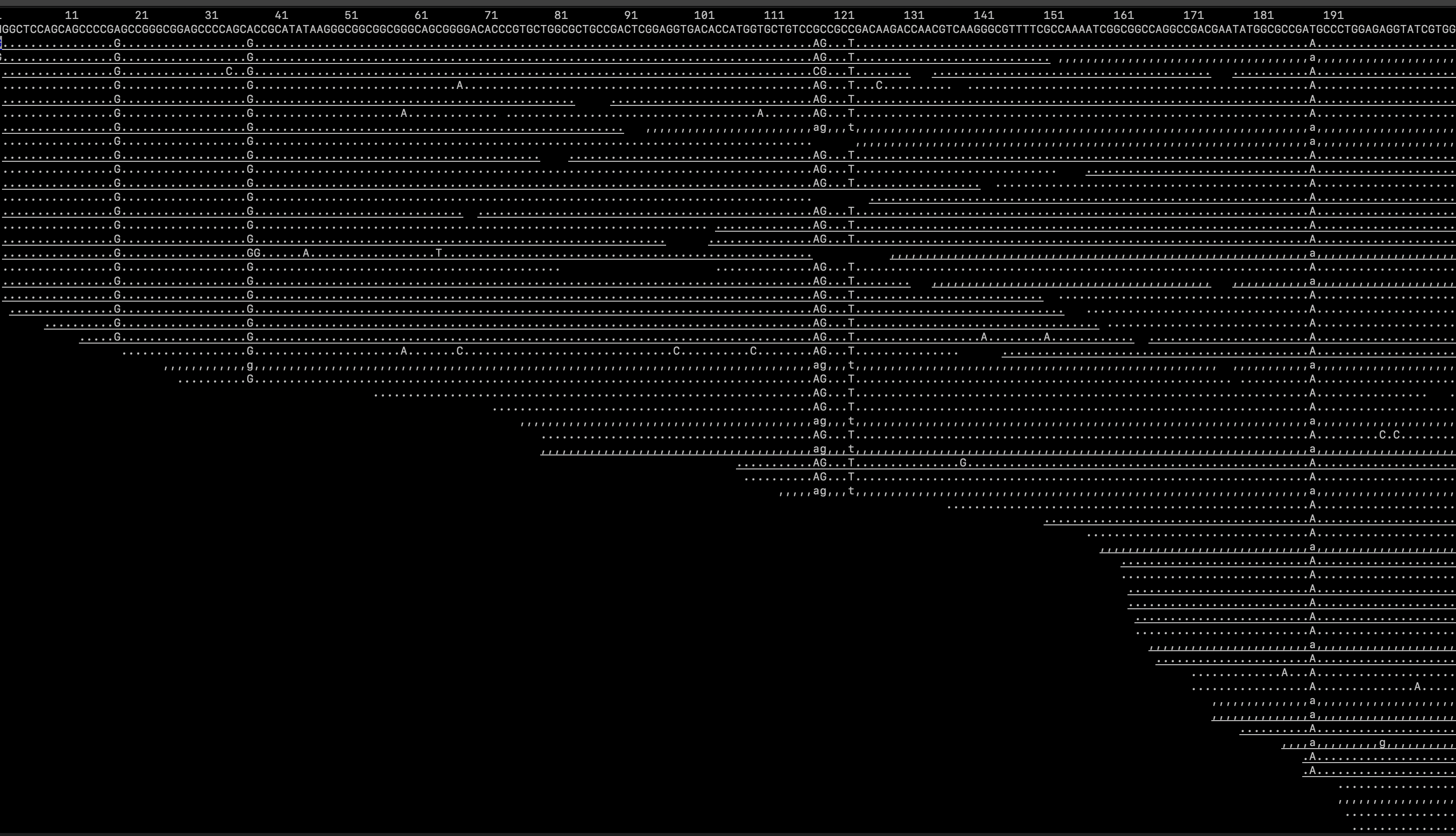
samtools tview sample.sorted.bam hemoglobin_references.fastaUse the arrow keys to navigate this visualization, typing q to exit as needed. The top line shows the reference sequence; matching characters on the forward strand are shown as periods (.), while matching characters on the reverse strand are shown as commas (,). Nucleotides are only shown where one or more reads differ from the reference sequence; gaps in the alignment (or where reads were broken to improve their mapping) are shown as spaces. Hopefully you find this as satisfying as I do. The tview command has additional options, which you can read about in the documentation; leaving out a path to a reference sequence will show all nucleotides, for example, while the -p flag will open the alignment at the specified position.
samtools tviewLastly, we should examine mapping statistics. Both of the following commands are O.K. to run on the log-in node for this minimal dataset, but would be more safely put in a SLURM script / .sbatch file:
samtools flagstat sample.sorted.bam > alignment_stats.txt
samtools depth sample.sorted.bam | awk '{sum+=$3} END {print sum/NR}' > depth.txt
The former command produces a file called alignment_stats.txt with various alignment summary statistics; most important for our purposes is the percentage of reads mapped, found on line 7. (This will be very low, as the raw sequence data here includes many other regions of the genome beyond the seven hemoglobin subunits.) The latter command calculates depth of coverage, saving it to a text file named depth.txt. Examine both; you’ll be extacting info from them as part of today’s homework assignment.
As with last week, today’s homework has multiple goals:
- Successfully align all samples for your species to the same reference, either by pasting and modifying commands in sequence or using
.bashscripting tricks such as loops (e.g., the example provided in Homework 4); - Edit the structure of your subdirectory on the cluster to organize trimmed reads, sequence alignments, scripts, and notes in a logical and coherent manner;
- Create a Markdown file that contains the percentage of reads mapped and depth of coverage for each sample in your focal species dataset;
- Add, commit, and push this summary and all
.sbatchscripts used to your GitHub repository, again editing subdirectory structure and yourREADME.mdfile as necessary. (If you are pushing directly from the cluster, be careful not to try to upload raw data or alignment files!)