Demographic inference with dadi
A powerful an important use of genome-wide DNA sequence data is inferring the history of populations with statistical models. Though approaches to this problem (known as demographic inference) vary, they typically use either equations or simulations to generate expected patterns of genetic variation under user-specified scenarios, then assess the probability of these data (under a likelihood-based framework) or the posterior probability of a model (under a Bayesian framework) while simultaneously estimating parameter values. A typical workflow involves developing a set of plausible models with a relationship to your scientific hypotheses, generating summary statistics from these models and details of your population and genomic sampling, and then fitting your data to the model with some sort of optimization algorithm. You can then compare support for alternate models, interpreting the parameters of the one that provides the best match for your data.
Like many topics in this class, rigorously implementing demographic inference software requires thinking carefully about your system, extensive troubleshooting, and replication. We will avoid the most onerous of these tasks with a simple application of dadi to a simulated population bottleneck. The program’s documentation includes extensive discussion of many issues we will gloss over and additional examples; I encourage you to familiarize yourself with it.
Working with Jupyter Notebooks
Like snakemake, dadi is a Python-based tool. Because developing and evaluating models is substantially easier in a setting where you can run code line-by-line, we will work with the program in Jupyter, an application for interspersing interactive coding “chunks” with Markdown-formatted text (much like Rmarkdown). Before opening a new notebook file, however, we need use the command line to install the necessary software into a mamba environment that is accessible to Jupyter on tempest. Create a new .yaml with the following programs:
name: dadi
channels:
  - conda-forge
  - bioconda
dependencies:
  - python=3.11
  - dadi
  - msprime
  - tskit
  - numpy
  - scipy
  - matplotlib
  - ipykernel
  - pandas
mamba env create -f dadi.yamlWe now need to register this environment as a kernel (a process with access to a specific programming language and certain software), which will require activating the new environment and running a Python configuration command:
mamba activate dadi
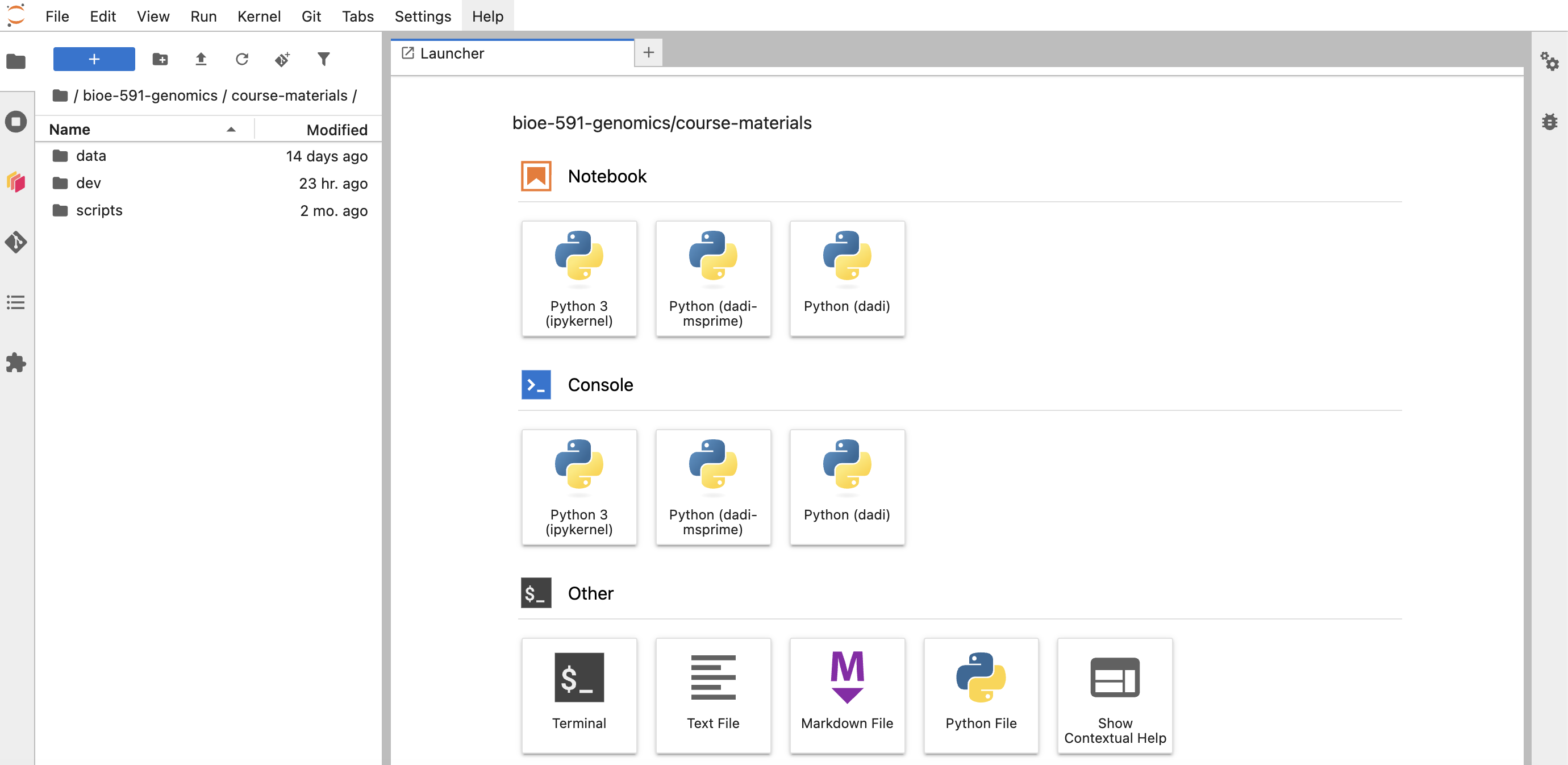
python -m ipykernel install --user --name dadi-msprime --display-name "Python (dadi)"Once this is done, use your browser navigate to the Tempest Web interface, log on, and navigate to Apps > All Apps. Click on JupyterLab. You will see the familiar prompt for requesting resources; adjust the runtime field as needed, and launch. Once the session has started, you should see a file browser pointed to your home directory on the left, while to the right is a pane labeled “Launcher”. At the top, you should see a tile labeled “Python (dadi)”. Click this—it will then open a new notebook running the kernel you installed above.
 This notebook will be named
 Untitled.ipynb, and be empty other than a field highlighted in blue at the top of the document. Click in this box, and navigate directly above your pointer to the dropdown box that reads “Code”. Click this, and select “Markdown”. You have now instructed Jupyter to interpret this “chunk” of the document as Markdown formatted text. To see the implications of this, give your document a header by entering hashtag(s) and plain text in this field (i.e., type ## Dadi Lab or similar). Click the forward-facing arrow near the dropdown box now reading “Markdown” (or enter Command + Return (⌘+↩︎) on your keyboard) to run (= evaluate) its contents. You should see it immediately formatted as if rendered to .html.
Running code works similarly. Add a new chunk below your headed, and enter the following:
two = 2
three = 3
two*three
Clicking run should print 6 to your console as the multiplication operator * is applied to objects with stored integer values. But what if you’d like to start over, clearing all output and assignments? You can do so by clicking the circular arrow button next to the square “stop” icon, or by navigating to “Restart Kernel…” under the “Kernel” dropdown menu.
That’s really all there is to it—you are now familiar with the core functionality of Jupyter! For the remainder of the tutorial, alternate between Markdown and Code chunks to annotate, enter, and execute lines from the scripts presented below. More detailed introductions can be found here and here; refer to both as needed throughout the exercise.
Simulating sequence data with msprime
An exciting frontier in population genetics is the development of an ecosystem of Python libraries for efficiently simulating and analyzing genetic data. Many of these libraries use a novel data structure called a tree sequence, which stores locus-specific ancestry and mutation information. Tree sequences underpin the program msprime, which simulates DNA sequences under user-specified evolutionary scenarios.
We will use msprime to generate a .vcf file containing variants from a population that underwent a severe bottleneck in the past. To start, we must load the relevant libraries (analogous to install.packages() in R). Note that you can use import <package> as <name> syntax to nickname it (useful for accessing modules and functions with fewer characters):
import msprime
import dadi
import numpy as np
We then create an object called demography with msprime’s Demography() function. Here, the period specifies the function belongs to a particular library:
demography = msprime.Demography()One feature of Python that is distinct from R is that objects themselves can have methods, or functions specific to their contents. The .add_population() and .add_population_parameters_change() methods thus modify the demography object (essentially a representation of your model) by 1) creating a population with a present-day size of 500 and 2) specifying that it originated from an ancestral population of \(N_e\)=10,000 that was bottlenecked 800 generations previously.
demography.add_population(name="pop", initial_size=500)  # present size

# ancestral size before T=800 generations ago was 10,000
demography.add_population_parameters_change(
    time=800, initial_size=10_000, population="pop"
)
(Note that in Python 10000 and 10_000 are equivalent; the latter is simply a more human-readable version of the former known as a numeric literal separator)
Entering demography should print a table including salient features of your model. We next describe the simulation itself with the .sim_ancestry function. Here, you’ll see that we specify we are taking 20 samples (by default, 40 diploid individuals) of a population with demography specified by the model demography. For each of these samples, we simulate a 5 million base-pair sequence, with a recombination rate of \(1*10^-8\) (per unit sequence, per unit time):
ts = msprime.sim_ancestry(
    samples={"pop": 20},
    demography=demography,
    sequence_length=5_000_000,
    recombination_rate=1e-8,
    random_seed=42,
)
We next add mutations to the simulated ancestry at a rate of \(1*10^-8\):
mts = msprime.sim_mutations(ts, rate=1e-8, random_seed=43)This gives us our simulated genotypes, which can be viewed with the .genotype_matrix() method before being written to a file:
mts.genotype_matrix()
with open("bottleneck_sim.vcf", "w") as f:
    mts.write_vcf(f)
Check to make sure your working directory contains the intended .vcf. Once you have done so, you are ready to run dadi.
Working with dadi
Regardless of the source of your data, dadi requires you to assign individuals (as labeled in your .vcf) to the populations you intend to model. Using nano or another text editor, save the following as a file named pops.txt:
sample  pop
ind_0   pop
ind_1   pop
ind_2   pop
ind_3   pop
ind_4   pop
ind_5   pop
ind_6   pop
ind_7   pop
ind_8   pop
ind_9   pop
ind_10  pop
ind_11  pop
ind_12  pop
ind_13  pop
ind_14  pop
ind_15  pop
ind_16  pop
ind_17  pop
ind_18  pop
ind_19  pop
We can read this in along with our .vcf and convert it into the format dadi expects:
vcf_file = "bottleneck_sim.vcf"
popfile = "pops.txt"
dd = dadi.Misc.make_data_dict_vcf(vcf_file, popfile)
Next, we summarize these data as a site frequency spectrum (folded, as we do not know which allele is ancestral versus derived without additional information). This object (fs) is “projected” down to 30 chromosomes, a technique that averages the calculated frequency of the minor allele over all possible \(n\)=30 subsamples to account for randomly distributed missing data. We also provide it the population labels from out popfile, and print its sample size and number of SNPs to the console:
fs = dadi.Spectrum.from_data_dict(
    dd,
    pop_ids=["pop"],
    projections=[30],
    polarized=False,   # folded SFS
)
print("Spectrum sample size:", fs.sample_sizes)
print("Segregating sites:", fs.S())
We now specify the models themselves. Developing an understanding of each line of code would require time and reading beyond our capacity. The important things to note are the structure of these function definitions (def name(arguments)), the fact that they return a site frequency spectrum object to compare to your empirical data, and that we are comparing a null model of a single population of constant size (snm) to a model of a population size change some time in the past (two_epoch). This second model has two free parameters: nu, which is the size of the population at present relative to the size of the ancestral population, and T, which is the time (in units of \(2Ne_{\text{ancestral}}\) generations before present) of the population size change. The object phi (or \(\phi(x)\)) is the distribution of the number of polymorphic sites with a particular allele frequency; xx is the number of grid points used to approximate the curve of \(\phi\) (a larger value means greater accuracy but slower runtime):
def snm(params, ns, pts): # define single population model, no free parameters
    xx = dadi.Numerics.default_grid(pts)
    phi = dadi.PhiManip.phi_1D(xx)
    fs_model = dadi.Spectrum.from_phi(phi, ns, (xx,))
    return fs_model

def two_epoch(params, ns, pts): # define bottlenneck model
    nu, T = params # two free parameters: scaled current pop size and time of split
    xx = dadi.Numerics.default_grid(pts)
    phi = dadi.PhiManip.phi_1D(xx)
    phi = dadi.Integration.one_pop(phi, xx, T, nu)
    fs_model = dadi.Spectrum.from_phi(phi, ns, (xx,))
    return fs_model
The next three lines do something a bit sophisticated: they use the values in pts_l to calculate phi three times at increasing grid resolution, then use the differences among those calculations to extrapolate what phi would look like at effectively infinite resolution. They then create new versions of the demographic models that perform this extrapolation automatically (named snm_ex and two_epoch_ex, respectively):
pts_l = [40, 50, 60]
snm_ex = dadi.Numerics.make_extrap_log_func(snm)
two_epoch_ex = dadi.Numerics.make_extrap_log_func(two_epoch)
It’s now time to fit these models to our data and compare the result. This is trivial for our null hypothesis of no popualtion size change: we take the extrapolated version of snm, indicate it has no parameters ([]), feed it the sample size from out empirical SFS, and give it the grid point values we input above. This produces an expected SFS under the constant-size model. Because this model describes only the shape of the spectrum, we then scale it to match the total diversity in our data by estimating the parameter \(\theta\) (\(=4N_e\mu\)). Finally, we compute the multinomial log-likelihood, which measures how well the shape of the model SFS matches the observed data.
model_snm = snm_ex([], fs.sample_sizes, pts_l)
theta_snm = dadi.Inference.optimal_sfs_scaling(model_snm, fs)
ll_snm = dadi.Inference.ll_multinom(model_snm, fs)

print("\nConstant-size model")
print("log-likelihood:", ll_snm)
print("theta:", theta_snm)
The process is more complex for our model of a population bottleneck, as we need to determine the best-fit parameter values before we calculate its log likelihood. To do this, we provide educated guesses for nu (here, 0.5, indicating a 50% contraction from its ancestral population size) and T (0.1, or \(0.1*2N_e\) generations in the past), give these estimates lower and upper limits, and randomly perturb their value within an order of magnitude of its input value (fold=1):
p0 = [0.5, 0.1]
lower_bound = [1e-3, 1e-4]
upper_bound = [20, 10]
p0_perturbed = dadi.Misc.perturb_params(
    p0, fold=1, lower_bound=lower_bound, upper_bound=upper_bound
)
We then use an algorithm (of which there are several choices) to traverse the multinomial likelihood surface and (ideally) find its global maxima. The the dadi.Inference.optimize_log() function does this with these perturbed parameters, the empirical SFS, and the model in question; maxiter specifies the number of iterations to run.
popt = dadi.Inference.optimize_log(
    p0_perturbed,
    fs,
    two_epoch_ex,
    pts_l,
    lower_bound=lower_bound,
    upper_bound=upper_bound,
    verbose=1,
    maxiter=50,
)
Finally, we fit the model with these optimized parameter values, scale it to \(\theta\), and calculate the likelihood:
model_two = two_epoch_ex(popt, fs.sample_sizes, pts_l)
theta_two = dadi.Inference.optimal_sfs_scaling(model_two, fs)
ll_two = dadi.Inference.ll_multinom(model_two, fs)

print("\nTwo-epoch model")
print("best params [nu, T]:", popt)
print("log-likelihood:", ll_two)
print("theta:", theta_two)
Comparing Akaike Information Criterion (AIC) scores allows us to assess model fit while penalizing models with more parameters (lower is better):
print("\nModel comparison")
print(f"Delta log-likelihood (two-epoch - constant): {ll_two - ll_snm:.3f}")

# constant model has k=0 free params in this formulation
# two_epoch has k=2
aic_snm = 2 * 0 - 2 * ll_snm
aic_two = 2 * 2 - 2 * ll_two

print(f"AIC constant: {aic_snm:.3f}")
print(f"AIC two-epoch: {aic_two:.3f}")
Lastly, we will want to see what the parameter values from our best-fit model actually are. The “true” parameters here are printed from what we input into msprime (nu = 500 / 10000 = 0.05; T = 800 / (2 * 10000) = 0.04); the inferred parameters are stored in the optimized popt object:
print("True parameters:")
print("nu =", 0.05)
print("T  =", 0.04)

print("\nInferred parameters:")
print("nu =", popt[0])
print("T  =", popt[1])
We can scale these to “real” units with a bit of math:
N_anc = 10_000  # known from simulation
nu_est, T_est = popt # label popt parameter estimates
N_curr_est = nu_est * N_anc # multiply Nu in dadi units by ancestral populaiton size to get current N_e
t_est = T_est * 2 * N_anc # multiply T in dadi units by 2N_e to get generations
print("Estimated current size:", N_curr_est)
print("Estimated bottleneck time (generations):", t_est)Today’s assignment simply requires you to add, commit, and push the Jupyter notebook you used to complete the tutorial to Github, with a short Markdown chunk interpreting the AIC scores and parameter values. Did dadi infer the correct model? Are the parameter estimates close? As usual, you’ll want to edit directory structure and README.md files appropriately.